Supervised learning
We are given training data $(X, Y) = \{(x_1, y_1 ),\cdots , (x_N, y_N )\}$
- X: independent variables, inputs, predictors, features
- Y: dependent variables, outputs, response
$x \in \mathbb{R}^P$ (usually)
- regression: $y \in \mathbb{R}$
- classification: $y \in \{0, 1\}$
- structured prediction: More complicated high-dimensional spaces with dependent components (e.g. the space of images or sentences)
We assume $y_i = f(x_i ) + \varepsilon_i$
$\varepsilon$ is noise (includes randomness and approximations)
- Independently and identically distributed (i.i.d.) according to some probability distrib. (e.g. Gaussian)
Given the training set $(X, Y)$, we want to estimate $f$:
- to study the relation between x and y
- to make predictions of y’s for unobserved x’s
Good predictors can be hard to interpret
Parametric learning
Index functions $f$ by a finite-dimensional parameter vector
E.g. linear regression
- Parameters are coefficients of a hyperplane
- Parameters have a clear interpretation
- Can be a bad approximation of reality
Linear regression
via the lm function in R
library('ggplot2')
DataIncm <- read.table('Data/Income2.csv',header=T,sep=',')
ggplot(DataIncm) + geom_point(aes(x=Education,y=Income))
fit <- lm(Income ~ Education, DataIncm); fit
The first argument is a formula
- takes the form response ~ predictors
- response is a linear combination of predictors
- above we have just one predictor: $Education$
- $Income = \beta_1 \cdot Education + \beta_0 + \epsilon$
Second argument unnecessary if variables in formula exist in current environment
See documentation for other optional arguments
Can print fit:
fit
This is not all the information in fit (why?)
- Try
typeof(),class(),str() - Try plotting it
print.default(fit)
Observe fit contains the entire dataset!
Can disable with model = FALSE option
Can directly plot with ggplot :
plt1 <- ggplot(DataIncm, aes(x=Education, y = Income)) +
          geom_point(size=2, color='blue') +
          theme(text=element_text(size=10))
plt1 + geom_smooth(method='lm', se=FALSE, #Disable std. errors
                   color='magenta', size=2)
Can regress against Seniority
fit <- lm(Income ~ Seniority, DataIncm)
Can regress against both Education and Seniority
fit <- lm(Income ~ Education + Seniority, DataIncm)
+does not mean input is sum of Educ. and Sen.
Rather: $Income = \beta_2 \cdot Seniority + \beta_1 \cdot Education + \beta_0 + \varepsilon$
For the former, use I:
fit <- lm(Income ~ I(Education + Seniority), DataIncm)
- $Income = \beta_1 \cdot (Seniority + Education) + \beta_0 + \varepsilon$
Prediction
fit <- lm(Income ~ Education + Seniority, DataIncm)
How do we make predictions at a new set of locations? E.g. (15, 60) and (20, 160)?
pred_locn <- data.frame(Education=c(15,20), Seniority= c(60,160))
predict.lm(fit, pred_locn)
edu_pred <- 10:25
sen_pred <- seq(0,200,10)
pred <- data.frame(Education=rep(edu_pred, length(sen_pred)),
               Seniority=rep(sen_pred, each=length(edu_pred) ))
p_val <- predict.lm(fit, pred)
pred$p_val = p_val
plt <- ggplot(DataIncm, aes(x=Education, y=Seniority,
                          color=Income))+
    geom_tile(data=pred, aes(x=Education, y=Seniority,
                                  color=p_val, fill=p_val)) +
    geom_point(size=1) + theme(text=element_text(size=10)) +
    scale_color_continuous(low='blue', high='red') +
    scale_fill_continuous(low='blue', high='red') +
    geom_point(shape=1,size=1,color='black') +
      guides(fill=FALSE) # Remove legend for 'fill'
plt
Specifying a model for lm
| Symbol | Meaning | Example |
|---|---|---|
| + | Include variable | x + y |
| : | Interaction between vars | x + y + z + x:z + y:z |
| * | Variables and interactions | (x + y) * z |
| ^ | Vars and intrcns to some order | (x + y + z)^3 |
| - | Delete variable | (x + y + z)^3 - x:y:z |
| poly | Polynomial terms | poly(x,3) + (x + y) * z |
| I | New combination of vars | I(x*y + z) |
| 1 | Intercept | x - 1 |
See documentation and http://ww2.coastal.edu/kingw/statistics/R-tutorials/formulae.html
Generalized linear model
A linear model with Gaussian noise is often inappropriate. E.g.
- response is always positive
- count valued response
- {0, 1} or binary-valued as in classification
A better model might be:
$ response = g (\sum_{i=1}^N \beta_i \cdot predictor_i) + \varepsilon$
$g$ is a ‘link’ function, $\varepsilon$ is no longer Gaussian
Can fit in R with glm() (see documentation)
Nonparametric methods
No longer limit yourself to a parametric family of functions
Much more flexible
Often much better prediction
Complexity of $f$ can grow with size of dataset
Often hard to interpret
k-nearest neighbors
Given training data $(X, Y)$
Given a new $x^∗$ , what is the corresponding $y^∗$?
Find the k-nearest neigbours of $x^∗$ . Then:
- Classification: Predicted $y^∗$ is the majority class-label of the neighbors
- Regression: Predicted $y^∗$ is the average of the $y$’s of the neighbors
3-nearest neighbors
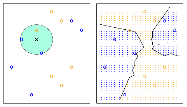 (*An Introduction to Statistical Learning*, James, Witten, Hastie and Tibshirani)
Complexity of decision boundary grows with size of training set: ‘Nonparametric’
Pros:
- Very intuitive computational algorithm.
- Very easy to ‘fit’ data (you don’t, you just store it)
- Tends to outperform more complicated models.
- Easy to develop more complicated extensions E.g. locally-adaptive kNN.
- Exists theory for such models.
Cons:
- Cost of prediction grows linearly with training set size (can be expensive for large datasets)
- Tends to break down in high-dimensional spaces.
- Exempler-based approaches are hard to interpret.
10-nearest neighbors
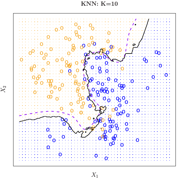 (*An Introduction to Statistical Learning*, James, Witten, Hastie and Tibshirani)
 (*An Introduction to Statistical Learning*, James, Witten, Hastie and Tibshirani)
- What distance function do we use? Typically Euclidean.
- What k do we use? Typically 3, 5, 10
Usually chosen by cross-validation (more later)
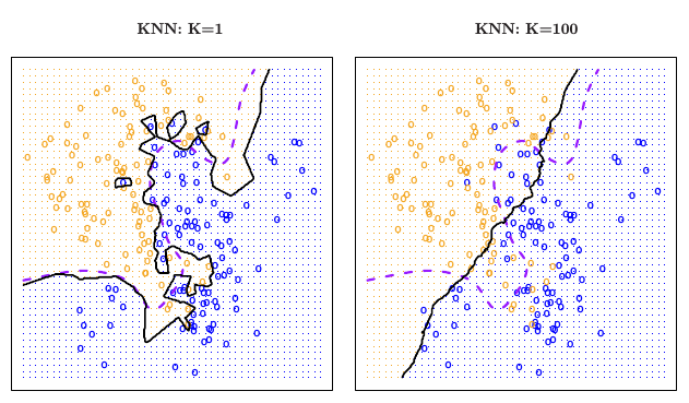
Large k: smooth decision boundary
Small k: complex decision boundary (with local variations)
- k is a measure of model-complexity
How do we perform model selection?
Do we prefer simple or complex models?
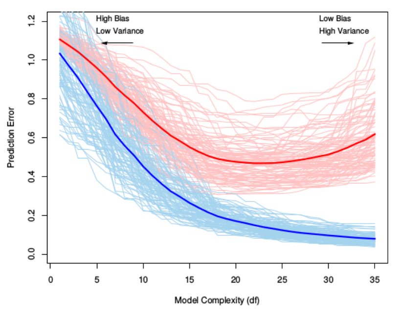
Bias-variance trade-off
Overly simple models
- cause underfitting (or bias)
- ignore important aspects of training data
Overly complex models
- cause overfitting (or variance)
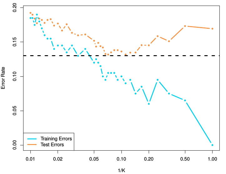
- can be overly sensitive to noise in training data
Complex models reduce training error, but generalize poorly.
Cross-validation
How do we estimate generalization ability? Create an unseen test dataset.
Cross-validation:
- Split your data into two sets, a training and test dataset.
- Fit all models on training set.
- Evaluate all models on test set.
- Pick best model.
Choosing k by cross-validation
Often 50-50 or 70-30 training-test splits are used
Too small a test set:
- Noisy estimates of generalization error
Too small a training set:
- Wasting training data
- Model selected using small training set may be simpler that model relevant to the entire training set
k-fold crossvalidation
Split your data into k-blocks.
For i = 1 to k:
- Fit algorithm on all except block i.
- Test algorithm on block i. Overall generalization error is the average of all errors.
- Can use larger training sets
- Can get confidence intervals on generalization error.
k = N: leave-one-out cross-validation
k-fold crossvalidation
 (*An Introduction to Statistical Learning*, James, Witten, Hastie and Tibshirani)